Written in early 2017 while the competition was running, and edited for clarity for this site. A few images that were hosted by Kaggle are no longer online and have been removed.
“Nearly half of the world depends on seafood for their main source of protein. In the Western and Central Pacific, where 60% of the world’s tuna is caught, illegal, unreported, and unregulated fishing practices are threatening marine ecosystems, global seafood supplies and local livelihoods. The Nature Conservancy is working with local, regional and global partners to preserve this fishery for the future.”
— from the competition page
The goal: how likely is each species in every picture?
Submission and evaluation
Submissions are evaluated with the multi-class logarithmic loss. Each image has been labelled with one true class, and for each image you submit a predicted probability for every class. The formula is
Target categories
Eight categories are available: albacore tuna, bigeye tuna, yellowfin tuna, mahi-mahi, opah, sharks, other (there are fish, but not of the above kinds) and no fish (no fish in the picture).
What makes it hard
Imbalanced fish types. Table 1 lists the number of images per type. For the detection pipeline and the classification pipeline alike, it is crucial to have a roughly balanced number of images per type — otherwise the network ends up biased towards certain fish (albacore, here) and the cute moonfish gets biased against.
| Code | Fish | Images | Share |
|---|---|---|---|
| ALB | Albacore tuna | 1,719 | 44.35% |
| BET | Bigeye tuna | 200 | 5.16% |
| DOL | Dolphinfish (mahi-mahi) | 117 | 3.02% |
| LAG | Opah (moonfish) | 67 | 1.73% |
| SHARK | Various sharks | 176 | 4.54% |
| YFT | Yellowfin tuna | 734 | 18.94% |
| OTHER | Other fish | 299 | 7.71% |
| NoF | No fish | 564 | 14.55% |
| Total | 3,876 | 100% |
Varied lighting. Day and night shots from the boats’ cameras look very different — more on that below.
Similar species — albacore vs bigeye (photos):
- Albacore tuna: an extremely long pectoral (side) fin that can reach past the first dorsal fin, up to the anal fin near the tail; a very dark upper body; a bright silver belly without vertical or horizontal lines; black finlets between the second dorsal fin and the tail.
- Bigeye tuna: the pectoral fin can pass the first dorsal fin, but is not as long as the albacore’s; a round body with vertical lines (adults) and stretch marks on the belly; a big head with big eyes; yellow finlets with a black border.
What makes it easier
One fish per image. Each image contains only one fish category — apart from the occasional very small fish used as bait.
The pipeline
1. Fish detection
Collecting images. Thanks to the collective effort of Kagglers, we had rectangular bounding-box and mouth-and-tail annotations from the very beginning, made with the annotation tool sloth. Because different people annotated, the mouth and tail can fall outside the rectangular box. For every annotated fish I also extract around ten background patches of the same size that do not overlap the fish.
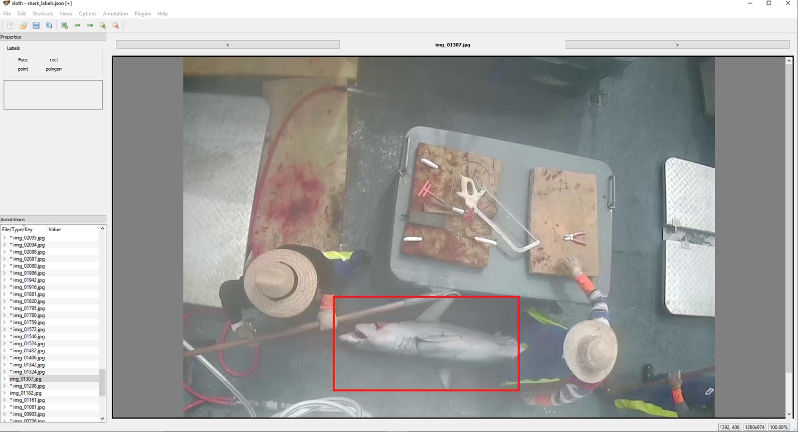
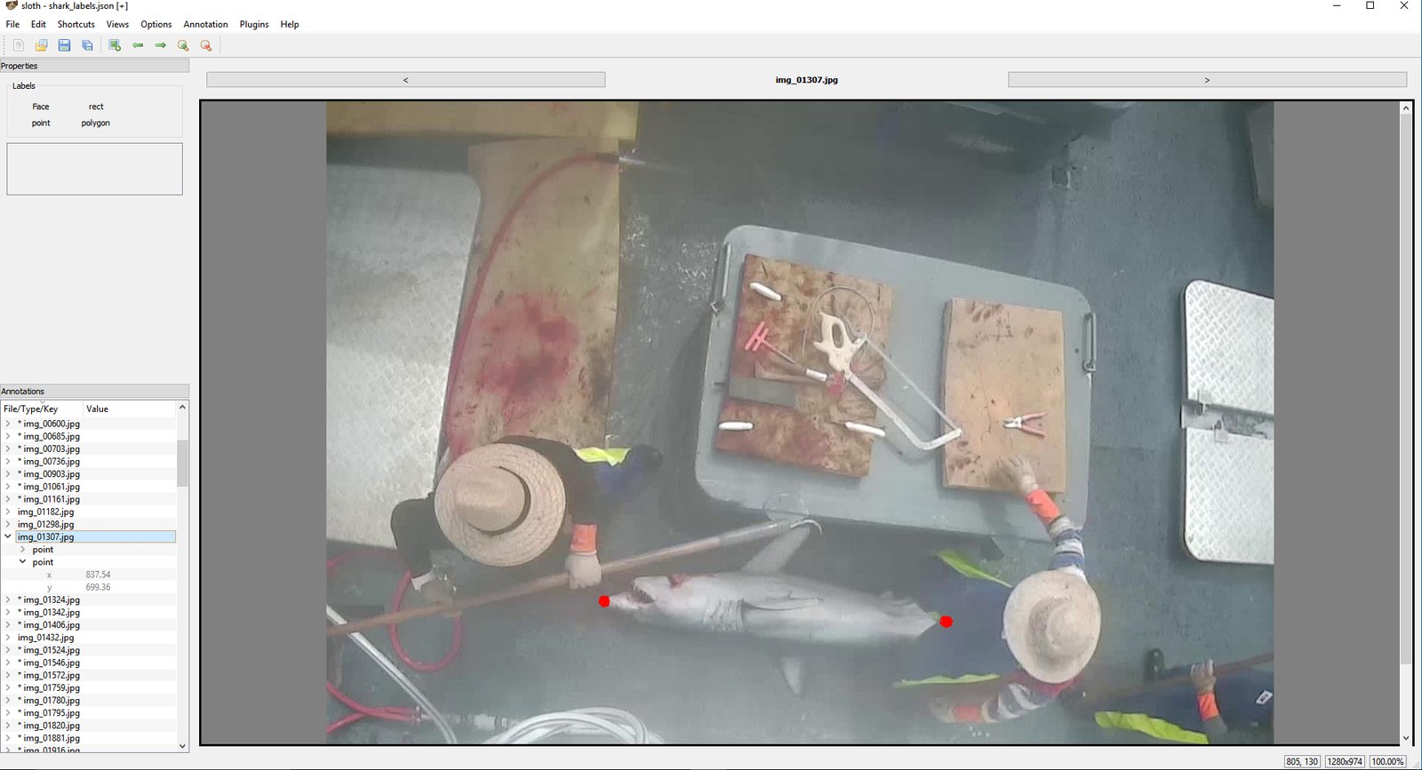
Annotations for the shark in img_01307. Left: rectangular bounding box. Right: mouth-and-tail annotation.
Training a bottleneck CNN. I went back to the good old HOG + SVM sliding-window approach from pedestrian detection: collect positive fish images and negative background (boat) images, following Building powerful image classification models using very little data. These are still natural images, so a network pretrained on ImageNet works directly, with a logistic regressor trained on top of the last convolutional layer. The average fish is about 180 × 180 pixels, but Keras’ ResNet-50 needs inputs larger than 197 × 197, so I always upsize the detector’s input to 200 × 200.
-
VGG19. I started with Keras’ pretrained VGG19; after 50 epochs (~100 seconds) the logistic regression reaches:
32716/32716 [==========] - 2s - loss: 0.0485 - acc: 0.9970 - val_loss: 0.1134 - val_acc: 0.9925 -
ResNet-50. As in the blog post above, ResNet’s last pooling layer gives features that generalise better:
32716/32716 [==========] - 1s - loss: 1.1921e-07 - acc: 1.0000 - val_loss: 0.0465 - val_acc: 0.9956
So ResNet-50 extracts the convolutional features for the rest of the experiments.
Hard negative mining, following the HOG + SVM pedestrian-detection pipeline.
Fine-tuning the convolutional layers. Next, the ResNet’s convolutional layers are fine-tuned, with data augmentation added to the binary detector:
ImageDataGenerator(rescale=1.,
                   featurewise_center=True,
                   shear_range=0.2,
                   zoom_range=0.2,
                   rotation_range=360,
                   horizontal_flip=True)
Training accuracy is much lower than for the bottleneck network because of the augmentation, and with every convolutional layer being tuned, training takes considerably longer:
11206/11206 [==========] - 527s - loss: 0.1217 - acc: 0.9580 - val_loss: 0.0295 - val_acc: 0.9898A fully convolutional detector. Turning fully connected layers into convolutions was proposed by Sermanet et al. 2014 and popularised by Long et al. 2015. Converting the last layer before pooling (a softmax layer) turns the trained binary fish classifier into a fully convolutional network (FCN), whose output is a heat map of whether each 56 × 56 grid cell holds a fish.
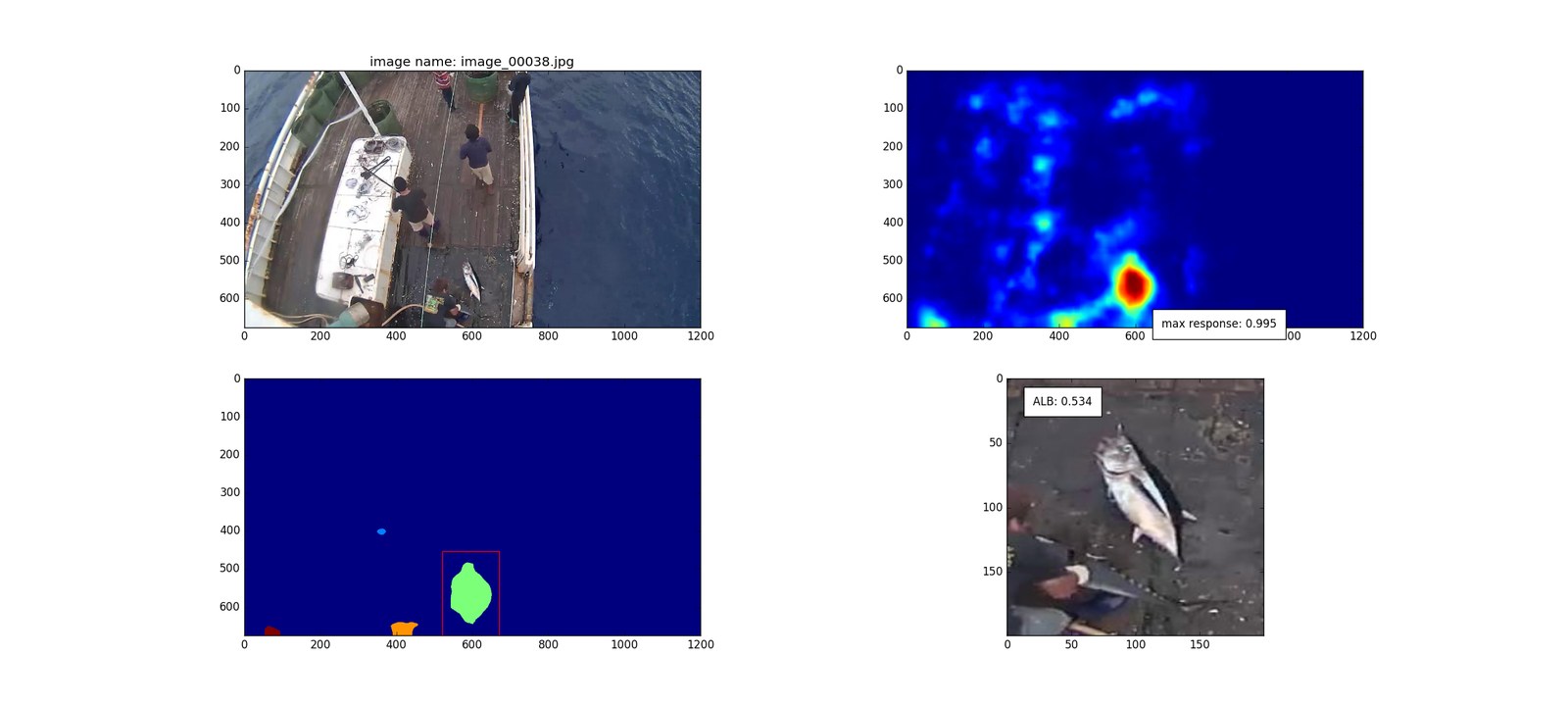
Multi-scale detection. Each output cell covers 56 × 56 pixels and fish vary a lot in size, so I run the FCN over several scales of the test image. The detector was trained on 200 × 200 inputs with fish of about 180 × 180, so I start from the original image size and scale it up by 1.1 eight times: nine response maps, from scale 1 to 1.1⁸ ≈ 2.14. As the illustrations below show, for a large fish (top) the smaller-scale maps respond more confidently, whereas for a small fish (bottom) the upscaled maps respond more strongly at the fish’s location.
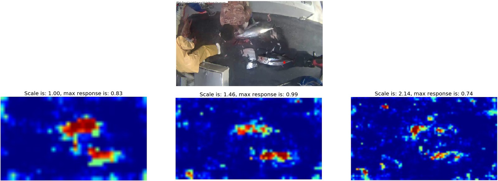
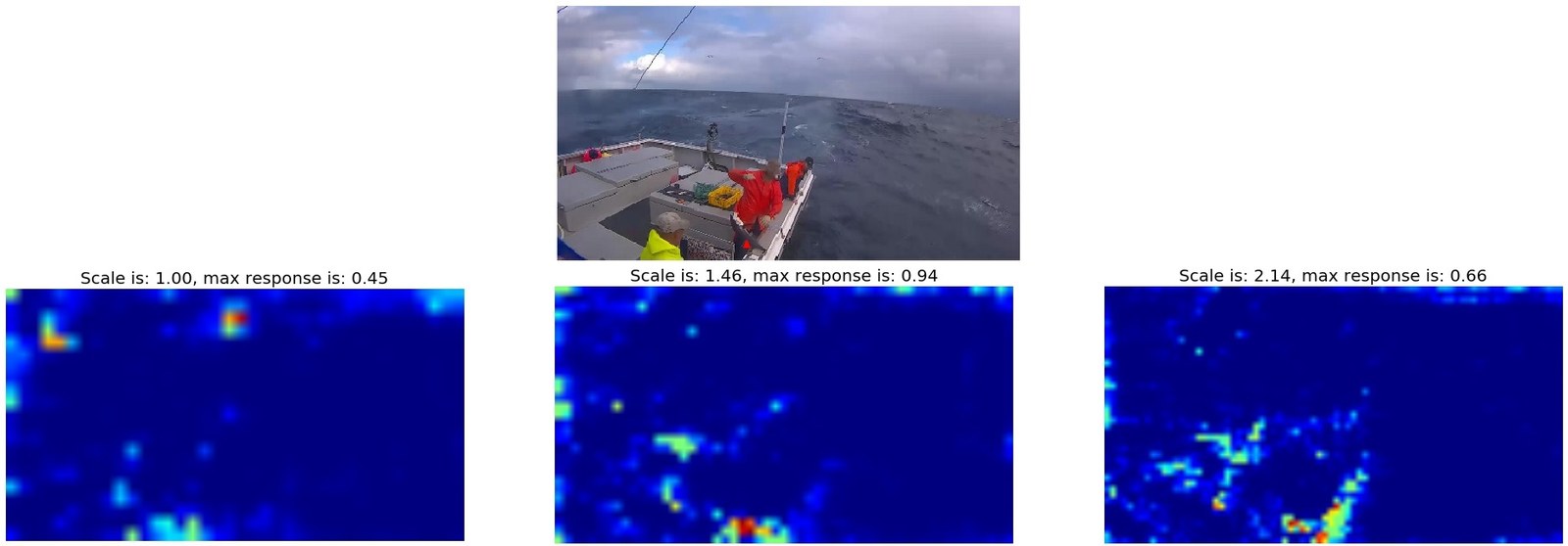
Response maps for different input sizes, upscaled to the original image size. For a larger fish (top) the smaller-scale map gives the stronger confidence; for a smaller fish (bottom) the upscaled maps do.
Attention map. Some areas near the image border respond very strongly because parts of the ship resemble the outline of a fish. I designed a heuristic attention map that damps the response near the left, right and top borders — but not the bottom, since salient objects can appear at the bottom of the frame but rarely at the top (the sky, for example). The figure shows it cleaning up false positives.
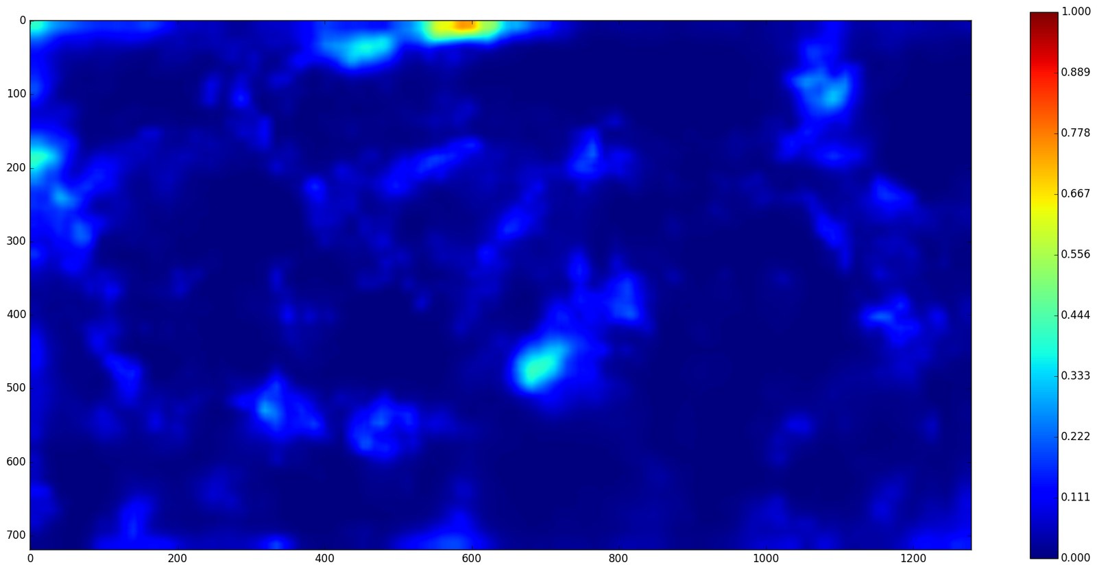
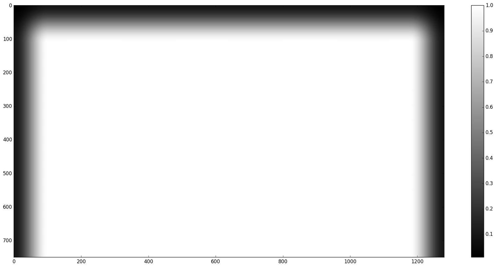
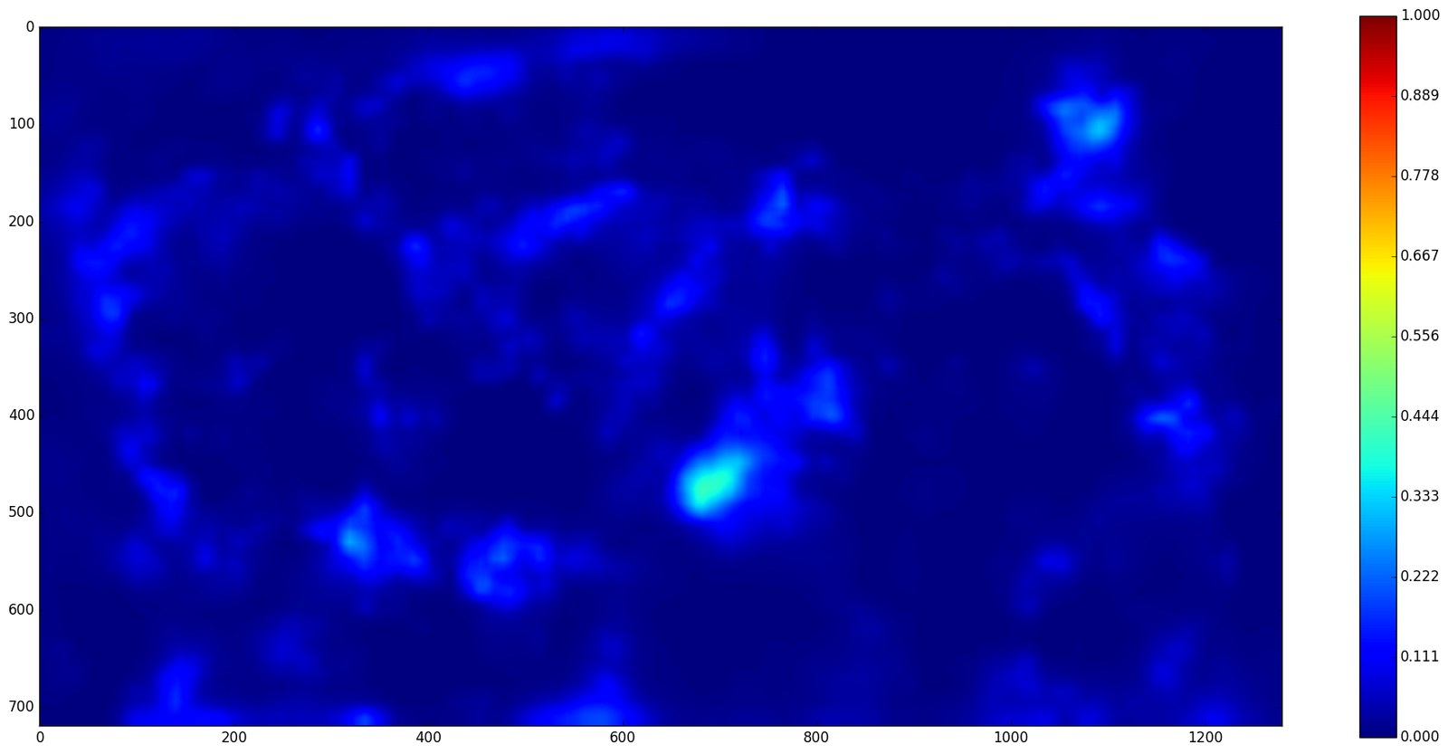
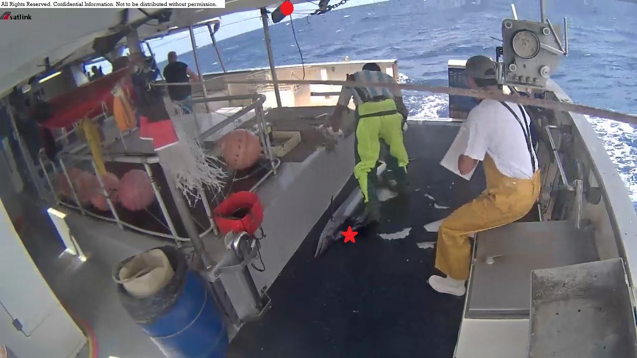
From left to right: (1) the original response map; (2) the attention mask; (3) the filtered response map; (4) with the original map, the most confident point (red dot) lands near the top of the image; with the attention map, the red star gets the higher salience score.
From response maps to boxes. Knowing that each image holds only one fish category, I take the maximum response as the centre of the fish, keep the connected region above a multiplying threshold, and expand it by a factor. A grid search using intersection over union (IoU) set the threshold to 0.4 and the expansion factor to 1.4. (A side note: in this IoU the predicted area counts only half, because slightly larger boxes help capture the whole fish — for fine-grained classification the details matter, and we want each detected fish to be as complete as possible.)

Response map, selected region and resulting crop for img_03547.
Evaluating detection. In PASCAL VOC, the highest-confidence box with 50% overlap counts as correct and all others as wrong; Hoiem et al. 2012 analyse detection errors in detail. Here I relaxed the criterion so that 30% overlap counts as a correct detection.
2. Fish alignment
I didn’t manage to align the fish the way the “Right Whale” challenge did, partly because the fish vary a lot here and the head and tail don’t always appear together. (Should we have? Perhaps a network could classify the fish and predict its head and tail locations at the same time.)
3. Fish classification
Fine-tuning ResNet-50. Again following Building powerful image classification models using very little data, applying a single network directly to the fish extracted by the detector gave my very first result:
The overall pipeline.

My first submission — with a rather disappointing ranking.
Clipping. The metric is cross-entropy, which punishes confident mistakes heavily, so I clip every prediction (log loss tricks, making sense of logarithmic loss):
where is a clipping variable, chosen heuristically as 0.95.
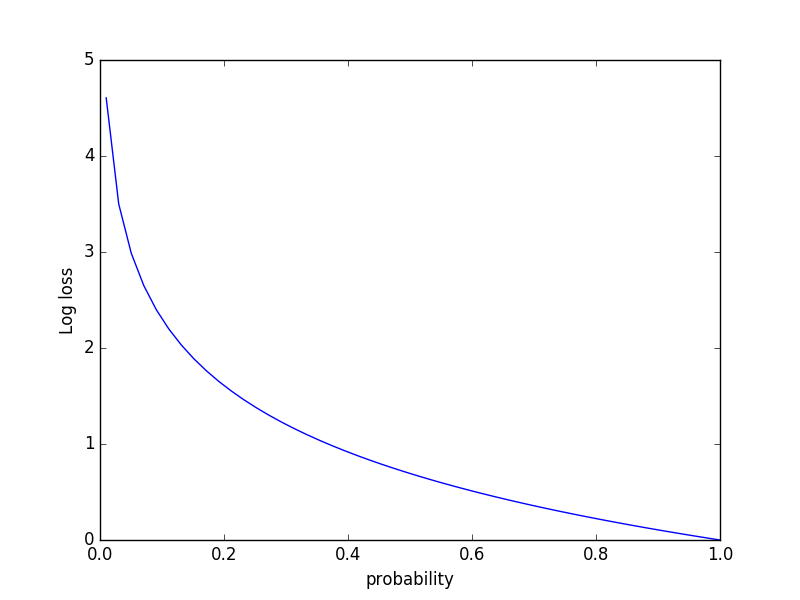
Log loss against the probability predicted for the true class.
Averaging over rotations. I also rotate each test image by 90° four times and average the predictions.
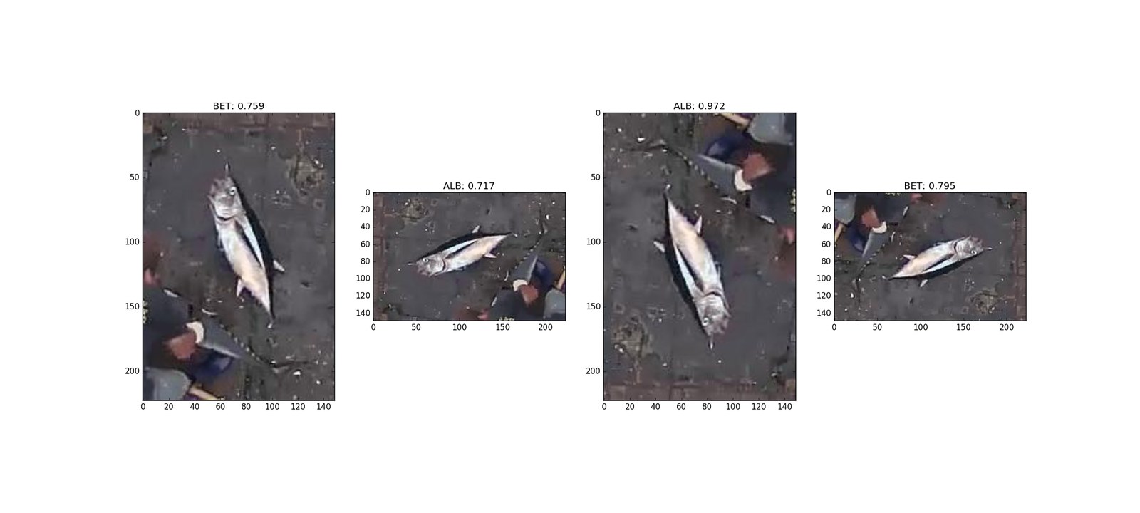
Rotated copies of an image can give very different results.
Day and night boats
Looking at the results, daytime boats with a “normal” colour cast are classified correctly and with high confidence. On night boats, with their yellowish cast, the classifier tends to put many fish into the yellowfin tuna (YFT) category — there are too few examples for the network to learn invariance to lighting. So I set out to train separate classifiers for day and night conditions.
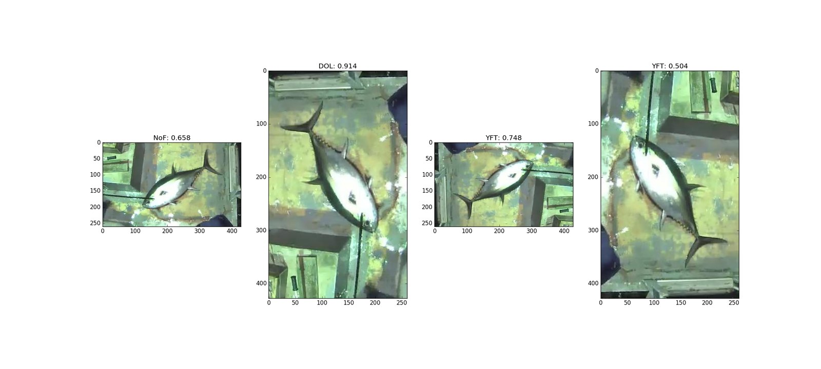
Incorrect labels caused by night-time lighting.
A holistic classifier
Albeit rather brute force, classifying the whole image works surprisingly well — sometimes better than the crops (discussion: worse performance on cropped images?). I suspect two reasons:
- Boat leakage: in this dataset the boat is strongly correlated with the kinds of fish it caught.
- Context: what surrounds the fish is itself a valuable cue for classifying it.
Ideas I didn’t implement, or couldn’t make work
- Right whale recognition by deepsense: for detection I actually started from their blog post, where whale detection uses the now-popular grid-based pipeline. I experimented with their code but couldn’t get the network to converge on this fishery data.
- DetectNet: deep neural-network object detection in DIGITS, whose data representation is inspired by Redmon et al. 2015.
References
- J. Redmon, S. Divvala, R. Girshick and A. Farhadi. You Only Look Once: Unified, Real-Time Object Detection. arXiv:1506.02640, 2015.
- J. Long, E. Shelhamer and T. Darrell. Fully Convolutional Networks for Semantic Segmentation. CVPR 2015.
- P. Sermanet, D. Eigen, X. Zhang, M. Mathieu, R. Fergus and Y. LeCun. OverFeat: Integrated Recognition, Localization and Detection using Convolutional Networks. ICLR 2014.
- D. Hoiem, Y. Chodpathumwan and Q. Dai. Diagnosing Error in Object Detectors. ECCV 2012, pp. 340–353.